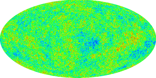
Planck 21 March 2013 based CMB radiation simulation - The Bubble Universe

The following three pictures are representations of the total sky.
Planck Scale 1 to 1
Temperature -514 to 517
Picture 1
Planck Simulation with large and small bubbles
Temperature -815 to 679
Picture 2
Planck Simulation with small bubbles
Temperature -904 to 684
Picture 3
The simulation of Picture #2 is performed by placing small temperature hills and valleys at random places on the surface of a sphere. This are the so called bubbles. The hills and valleys are placed in pairs. The size of each pair is the same. For a hill the temperature values are positif. For the paired valley the temperature values are the same but negatif. By doing this the average temperature value is kept (almost) constant. The initial average temperature is -44.
The simulation is performed by two types of hills and valleys (bubbles): large one's and small one's.
The total number of large one's (hills, valleys, bubbles) is 100000. The total number of small one's is 1000000.
The radius of the sphere of the simulation is 256 pixels. The radius of Picture #1,#2 and #3 is 128 pixels.

When you compare the picture #1 with picture #2 they are rather identical. The most important difference that Picture #2 does not contain any information about the physical state of the Universe.
Picture #3 shows only the small hills and valleys. This picture is important because in order to calculate the cosmological parameters only the large l values are used. See also . Reflection part 2

To observe the Power Spectrum based on Plank data, the Bubble Universe and WMAP data accordingly to the methode described at page 242 in the book "The Inflationary Universe" select this link: Critical evaluation of Power Spectrum calculation in the book "The Inflationary Universe" by Alan H. Guth


Reflection part 1

Document: Cosmological-Parameter Determination with Microwave Background Maps by G Jungman (23 May 1996) starts with the following sentence:
The angular power spectrum of the cosmic microwave background (CMB) contains information on virtually all cosmological parameters of interest, including the geometry of the Universe (Omega), the baryon density, the Hubble constant (h), the cosmological constant (Lambda), the number of light neutrinos, the ionization history, and the amplitudes and spectral indices of the primordial scalar and tensor perturbation spectra.
This is a rather astonishing sentence because the sentence only reflects the situation of Picture 1 but not of Picture 2.
The cosmic microwave background radiation (the temperature profile) can be described as a superposition of a dipole (l=2) a quadrupole (l=3) a octopole (l=4) and all types of multipoles until l=300 and higher. For difficulties involved to calulate the multipoles select: Low-order multipole maps of cosmic microwave background anisotropy derived from WMAP by P. Bielewicz K.M. Gorski and A.J. Banday (April 2004)

The problem is that electrical multipoles have a rather strict mathematical definition.
For example select The Static Electric Dipole, Quadrupole, & Multipoles by Professor K.E. Oughstun what is involved.
To get an idea about magnetic multipoles select:
Analytical Formulae For Magnetic Multipoles by M. Basetti and C. Biscari
The issue is that it is rather easy to calculate a field starting from a certain distribution, but very difficult to calculate the physical distribution (the source) starting from a distribution. That is what you want to do. You start from the cosmic micro wave background radiation and you want to calculate the multipoles that caused this radiation. What is more difficult the background radiation is a measurement on a sphere while the real cause is what happening in the inside and what is hidden. The remark can be made that what you try to do ie. starting from a sphere, has any physical bearing

To investigate this whole process in more detail consider the next: To calculate all these multipoles I expect is a very complicated task.

More to read:

The following three documents challenge the Planck results


Reflection part 2

The interpretation of the first peak in the CMB radiation is that the universe is flat.
See also The Mathematical Universe by Max Tegmark - Reflection part 3 - flat universe
See also Wikipedia CMB Primary anisotropy
The chalenge is to calculate the Power Spectrum of Picture #3 and to see what and where the peaks are. Because Picture #3 is based on hills and valleys of one pixel I expect that there will be only one peak. The radius of the sphere is 256 pixels.
The same exercise should be done for Picture #2.


Created: 23 April 2014

For more about the CMB radiation read this:

Back to my home page Contents of This Document